Introduction

Grasshopper is a “software inside another software”¹. It is a node-based visual editor that lets users build algorithms to generate complex geometries parametrically. Each node is a “box of math” that receives structured geometric data, transforms it, and sends the output to other nodes. This allows design through rules and relationships rather than fixed shapes, turning the process into dynamic and adaptable exploration.

Modeling Process (Conceptual Summary)

Before building the algorithm in Grasshopper, here is the overall flow:

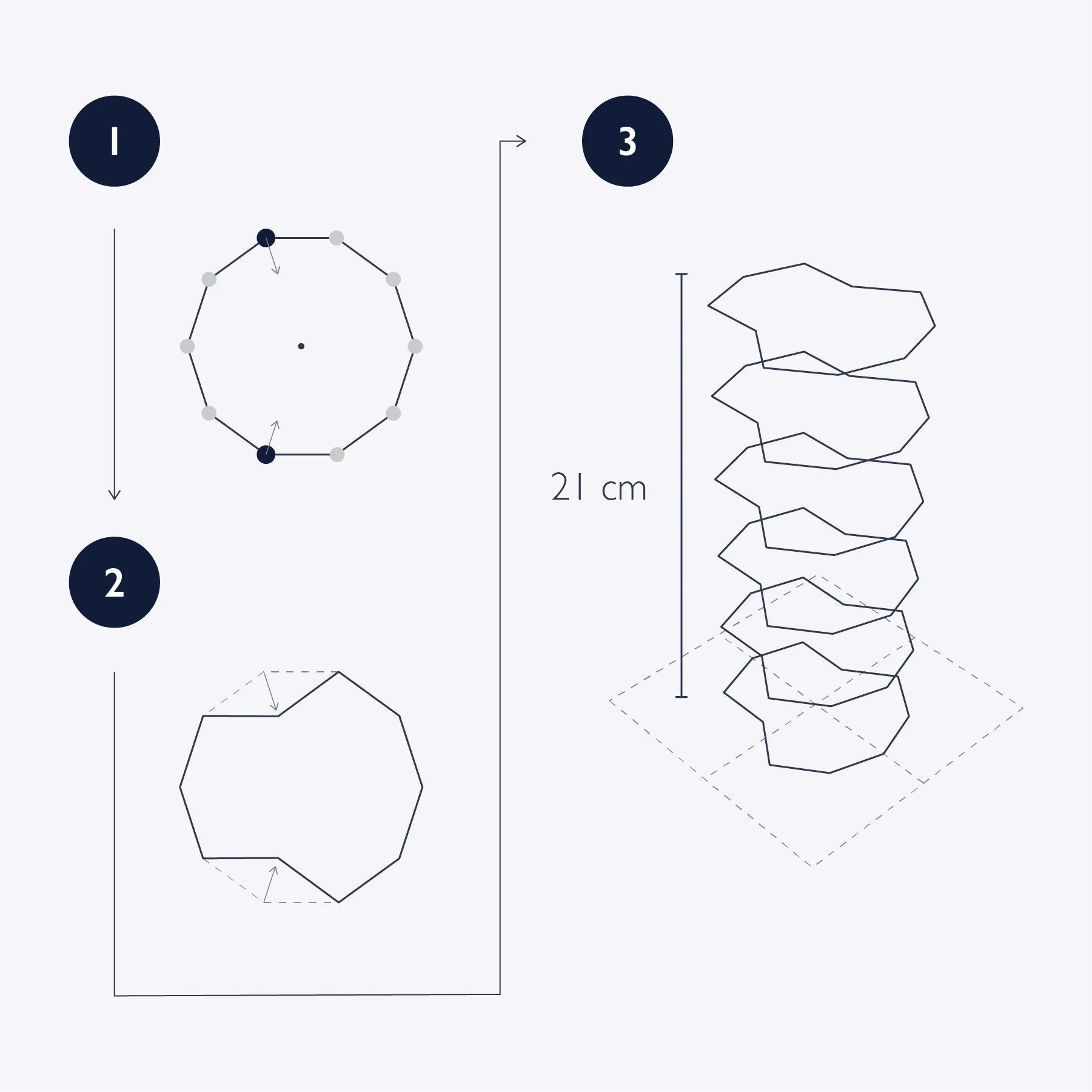
1. Start with a ten-sided polygon.
2. Move two vertices toward the center.
3. Stack copies of the modified polygon along the Z axis.
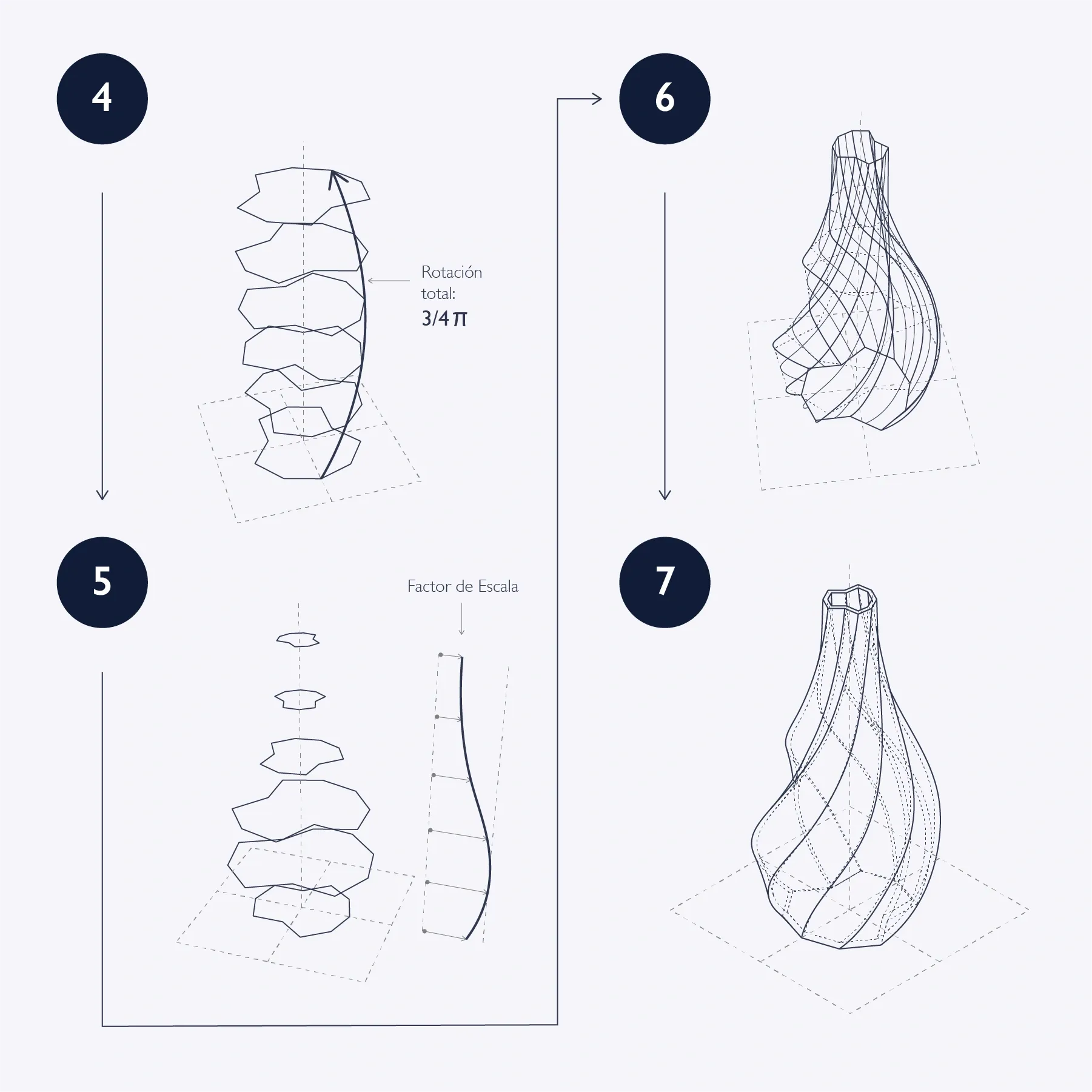
4. Rotate the resulting stack around the Z axis.
5. Apply variable scale to each stack level.
6. Perform a loft operation to create a continuous surface.
7. Add thickness to prepare for 3D printing.

As we build the algorithm, we can explore how parametric design enables fast variations by adjusting parameters (for example polygon side count or which vertices are moved), a key advantage over traditional modeling.

Building the Grasshopper Algorithm

Before opening Grasshopper, we confirm some Rhino settings: units in millimeters and grid size set to 220 mm (roughly our printer bed size on an Ender 3). In the screenshots below, Rhino is on the left and Grasshopper is on the right.

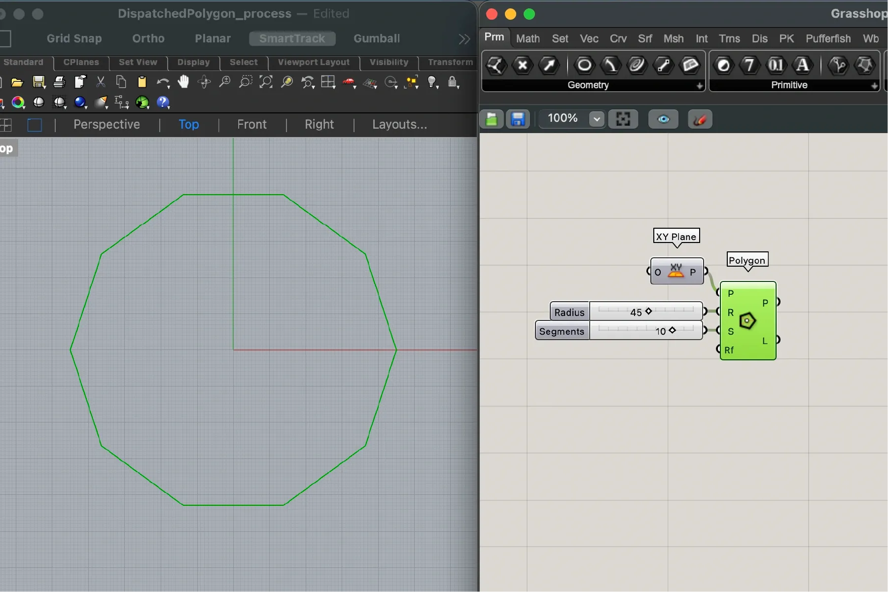
Initial Polygon

In Grasshopper, we start by creating a ten-sided polygon with the Polygon component. For this shape, we set a 45 mm radius and 10 sides via number sliders.

---

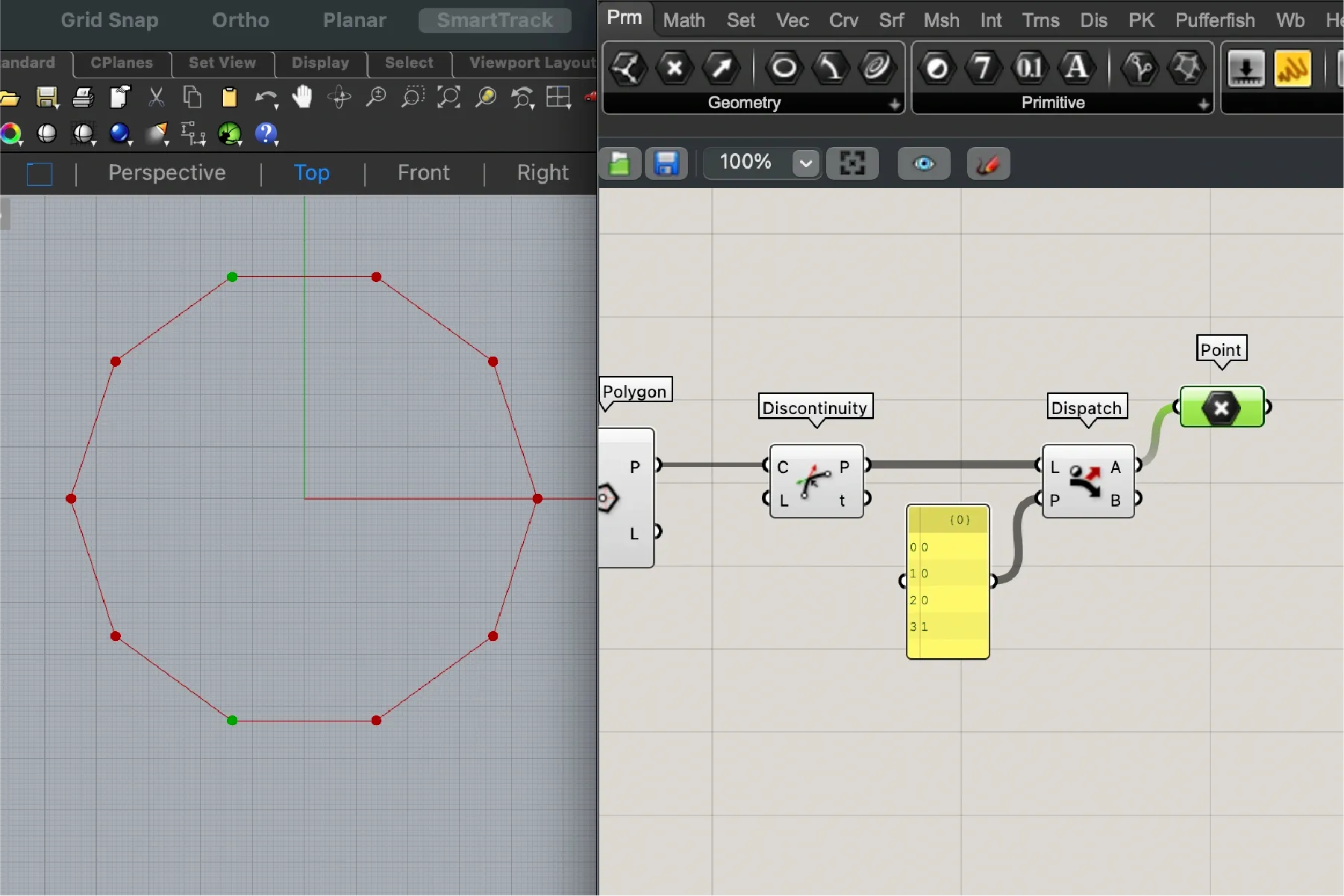
Splitting Vertices

The Discontinuity component extracts polygon vertices as a point list. Next, with Dispatch, we split these points into two lists using a boolean pattern²: one list keeps original-position vertices, and the other includes vertices that will move toward the center. In the image below, notice how the selected node highlights in green the two points isolated from the rest.

---

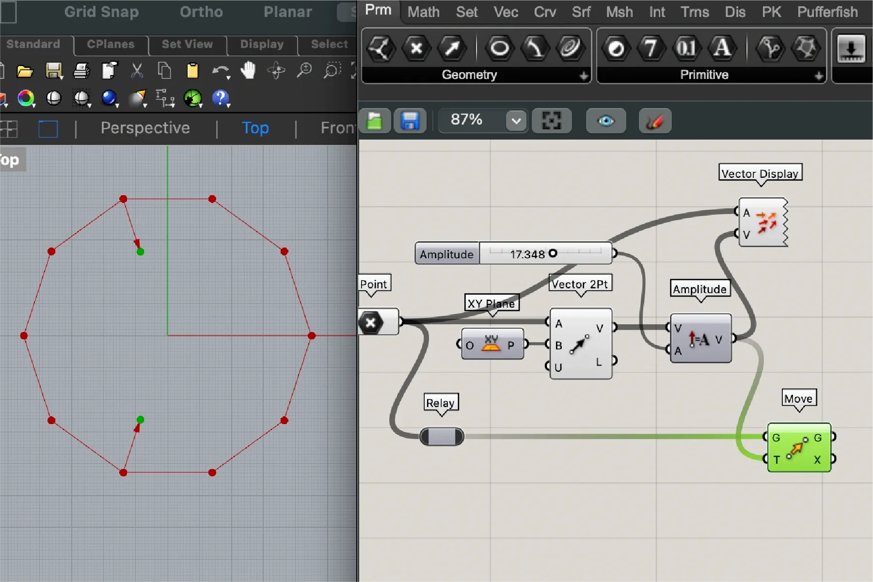
Vertex Translation

The Vector 2Pt component creates a translation vector from the selected points toward the center (coordinate origin). Then we assign vector magnitude with Amplitude (the connected slider controls how far points move). Finally, Move applies that translation to the selected points.

---

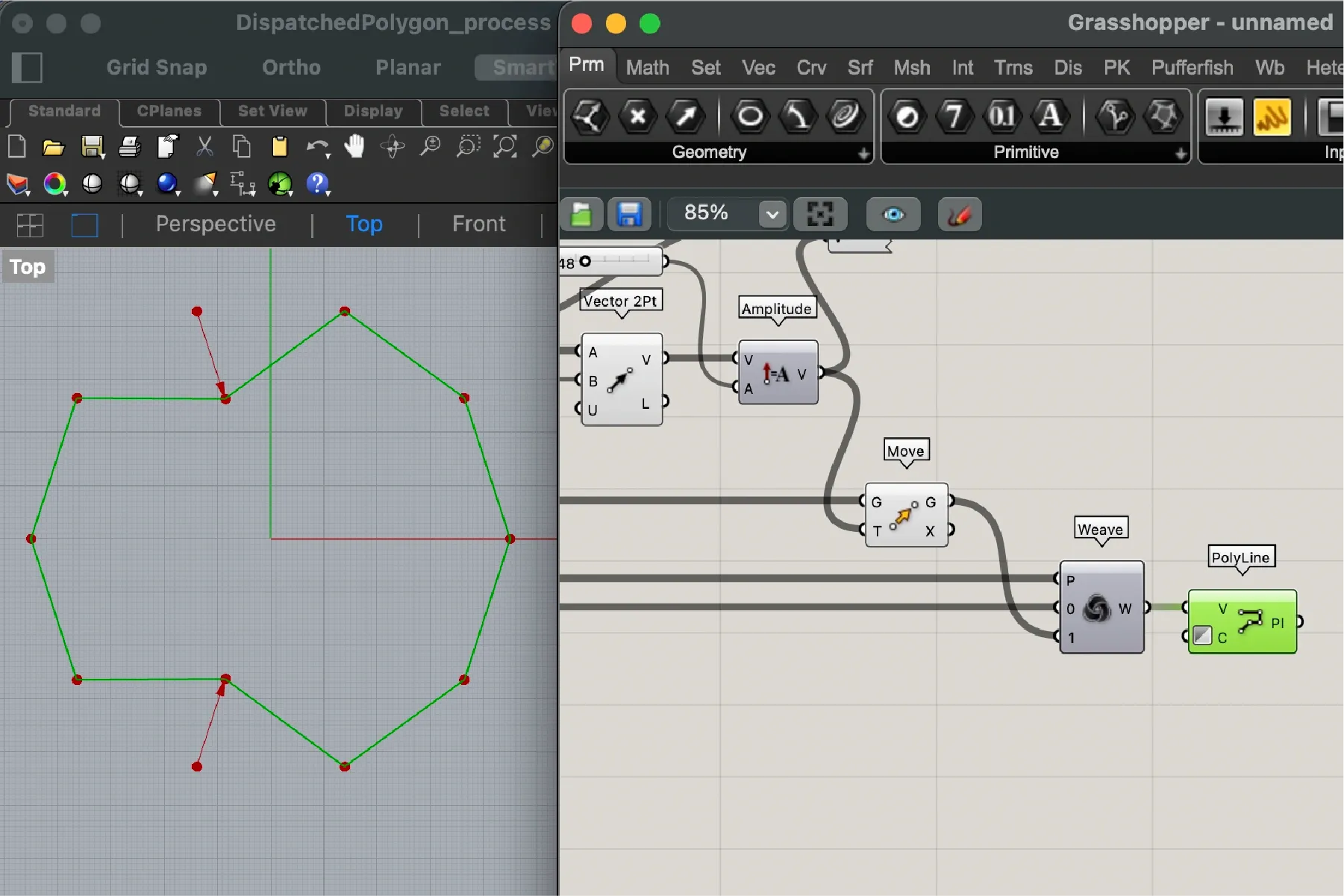
Polygon Reconstruction

The previous step only moved the two isolated vertices. Now we recombine moved and unmoved vertices with Weave, which receives both point lists plus the boolean pattern at input P. Then we rebuild the modified polygon with PolyLine. Input C (Closed) is toggled to create a closed polygon.

---

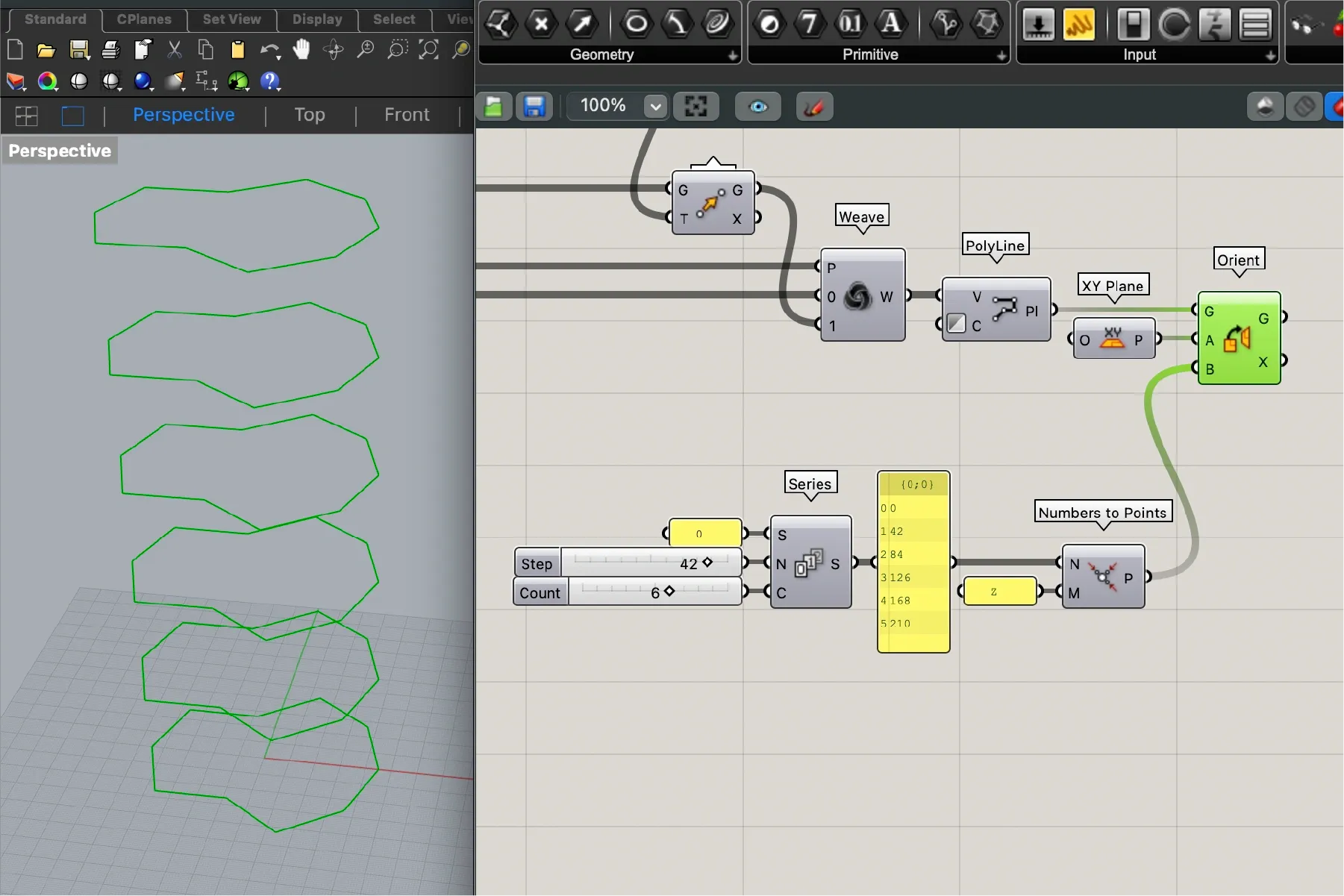
Stacking the Polygon

Next, we stack copies of the polygon. We begin with a numeric series using Series. This defines the heights (Z coordinate) for each copy. We set three parameters: start value (input S) at 0, step (N) at 42 mm, and count (C) at 6 levels. That means 6 copies, each 42 mm above the previous one along the Z axis. To position copies, we use Orient with that numeric series.

---

Rotating the Stack

Now we rotate the polygon stack. We use a similar method: another numeric series, this time generated with Range. This component defines values between min and max and lets us choose how many values we need within that range. Here, we need one the number of stack levels minus one³. A Graph Mapper could help us shape the spacing, but for this example we’ll just do a linear distribution. Then we multiply the values by pi (to define rotation angles in radians) and apply Rotate.

---

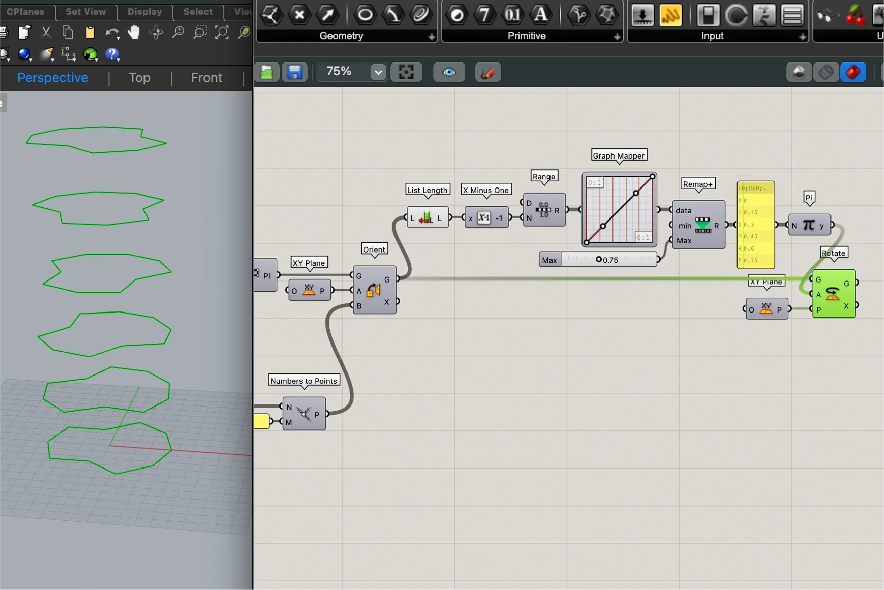
Scaling the Stack

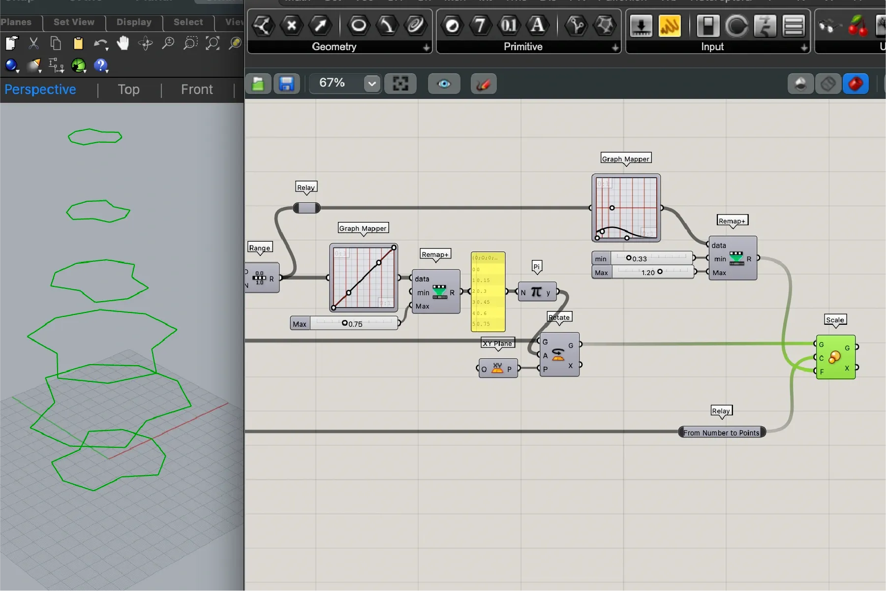
Once rotated, we apply a variable scale to each level. We reuse the previous range and feed it through a second Graph Mapper (Gaussian graph), which lets us manually shape scale values per level. To amplify the graph effect, we connect its output to Remap+, allowing us further control the transformation intensity. Finally, Scale applies the transformation.

---

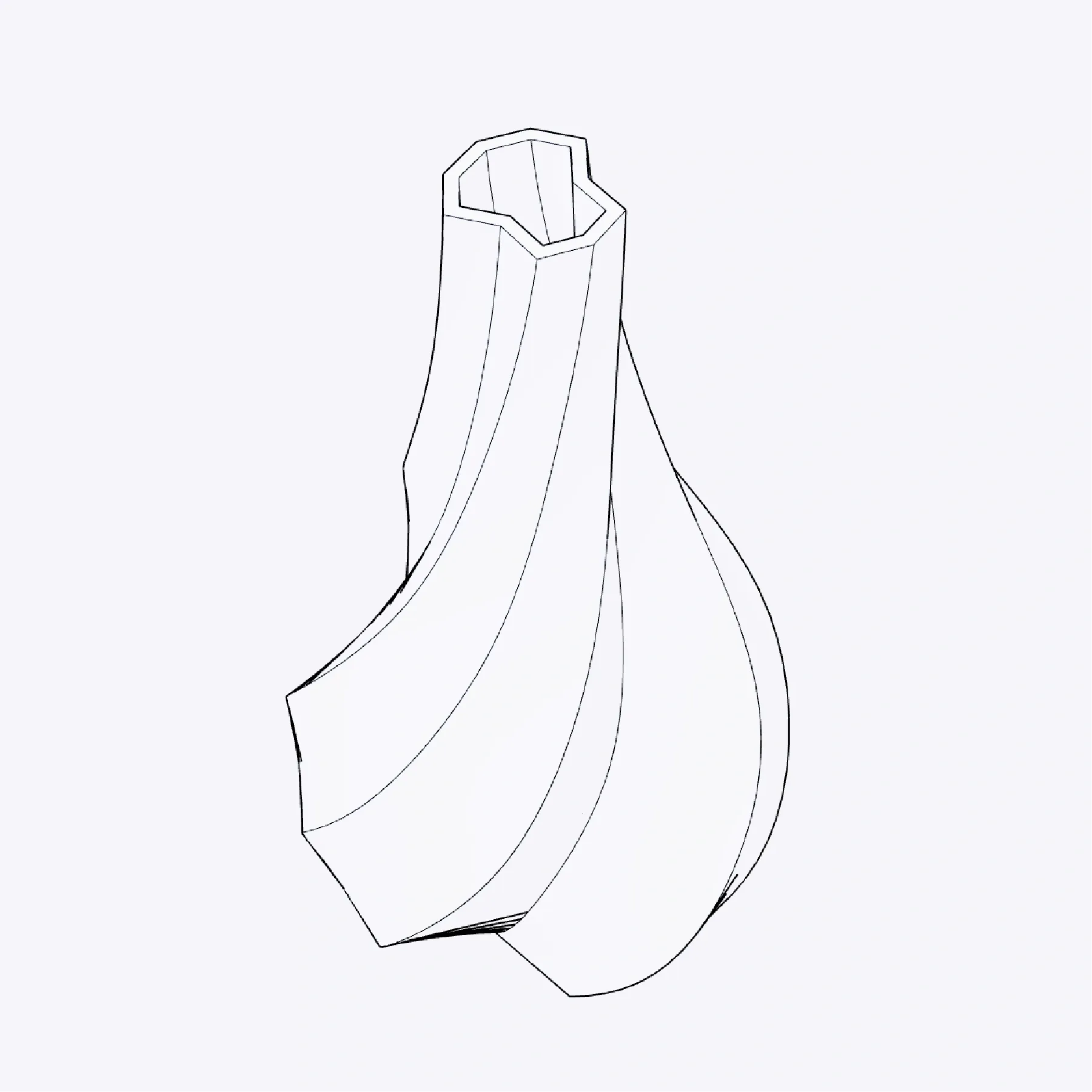
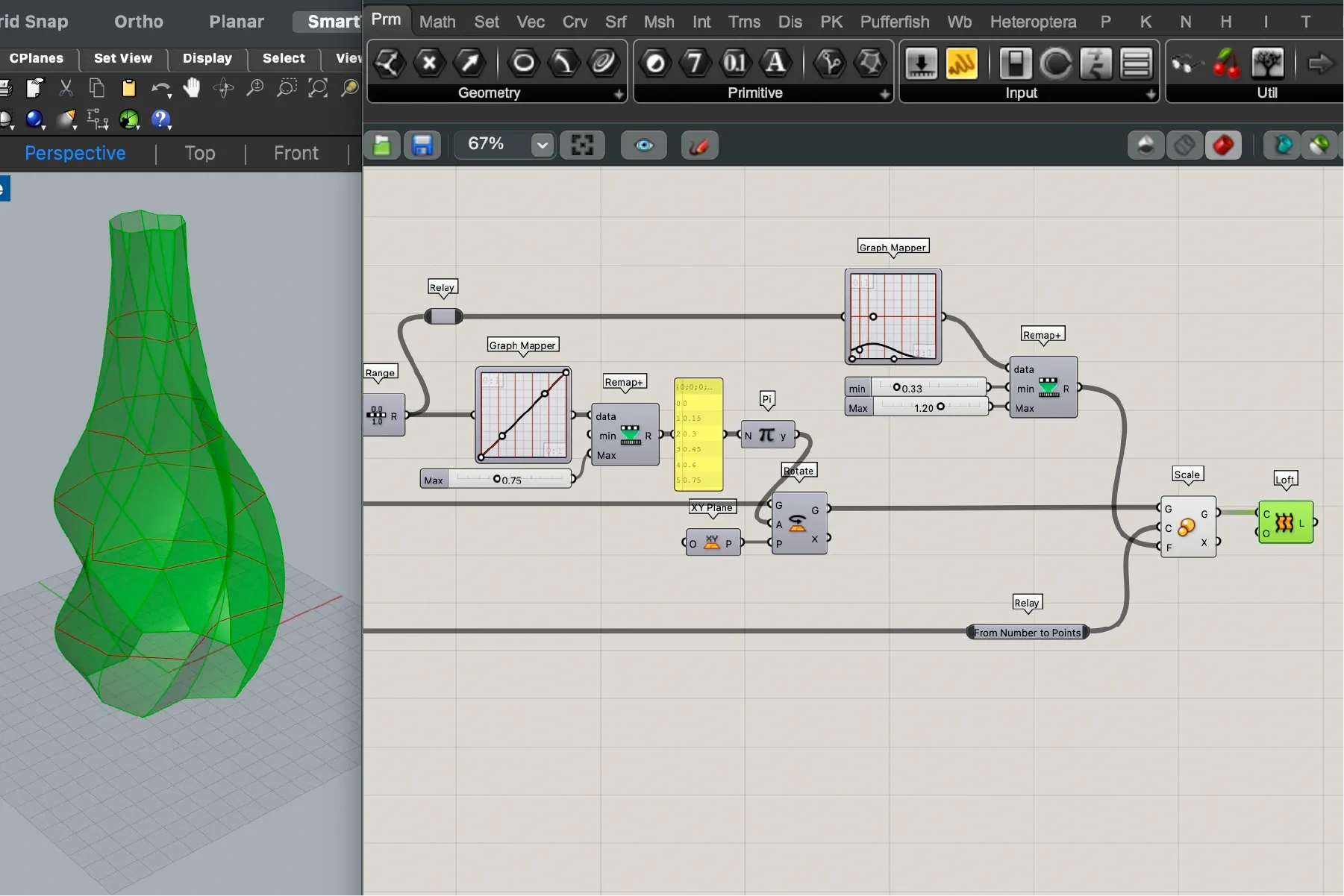
Initial Loft (Outer Surface)

At this stage, the base structure is complete. We can visualize the shape by connecting the stack to Loft, which creates a continuous surface between levels. To make the object printable though, we still need a few additional steps.

---

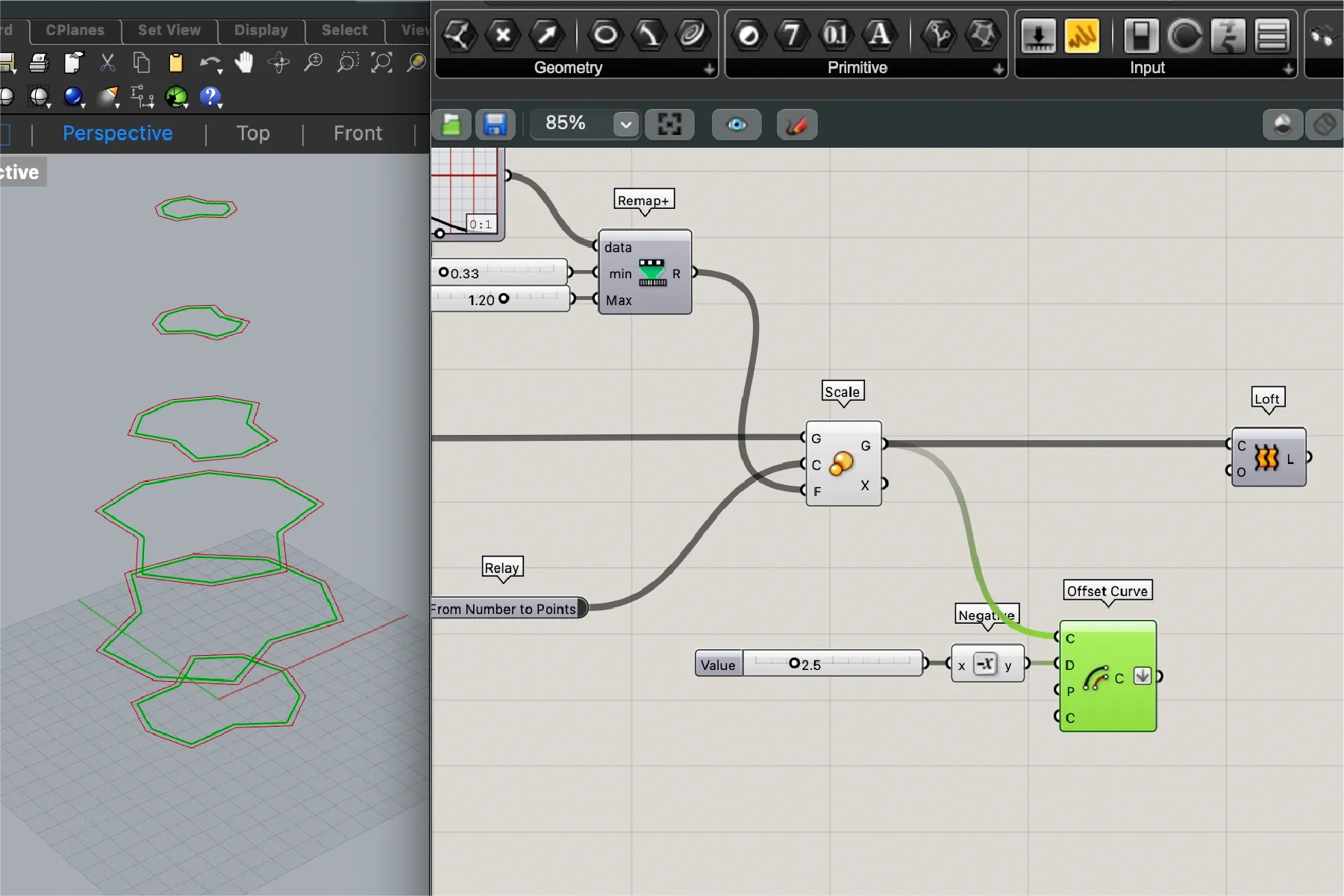
Offset (Inner Stack)

The Lofted surface has no wall thickness. For 3D printing, we need a solid. We start by sending the stack to Offset Curve with a negative value (-2.5 mm: the target wall thickness). This creates an “inner” stack shifted inward by that amount.

---

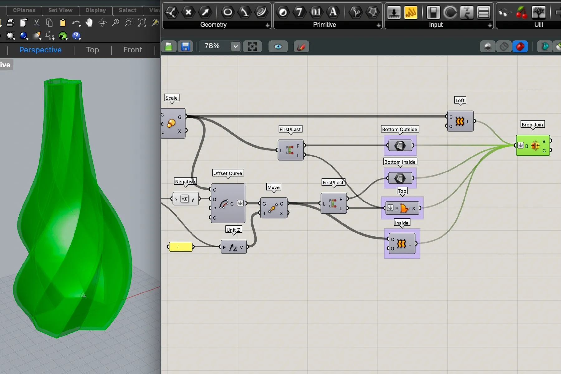
Inner, Top, and Bottom Surfaces

To form a closed solid, we create additional surfaces for final assembly. We begin by moving the first polygon of the inner stack upward by the same offset value (2.5 mm); this will create the base of the actual object. Then we loft between offset polygons to create the inner surface. We select the top two polygons (from original and offset stacks) and use Boundary Surfaces to create the top cap. The outer base polygon is already in place, so we only need to send it to a surface container to create the bottom cap.

---

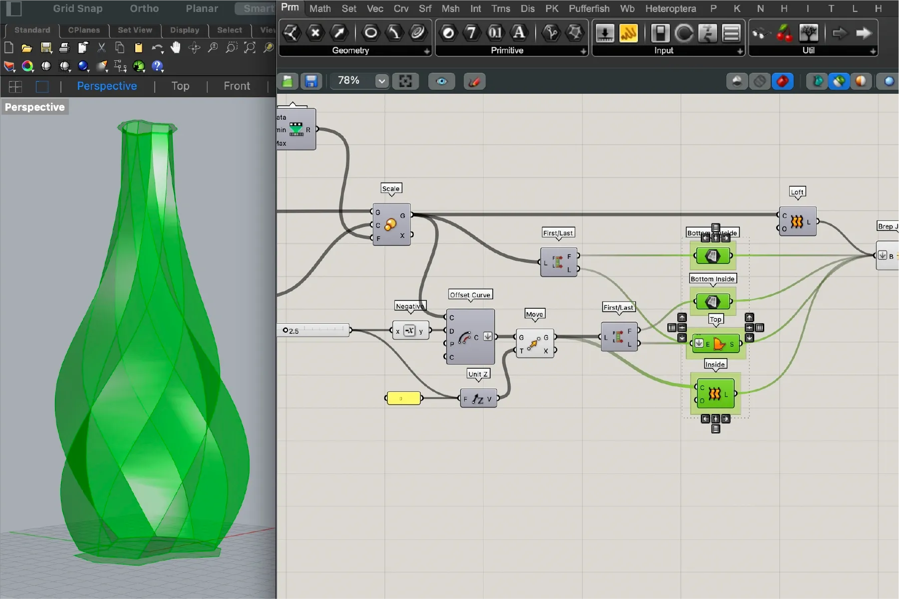
Completing the Solid

With all surfaces created, we use Brep Join to merge them into a single closed solid. Some components (such as Boundary Surfaces) output a tree (list of lists), so we flatten inputs where needed. We also flatten the Brep Join input to ensure all surfaces join correctly. The output is a Closed Brep: a sealed solid ready for STL export.

---

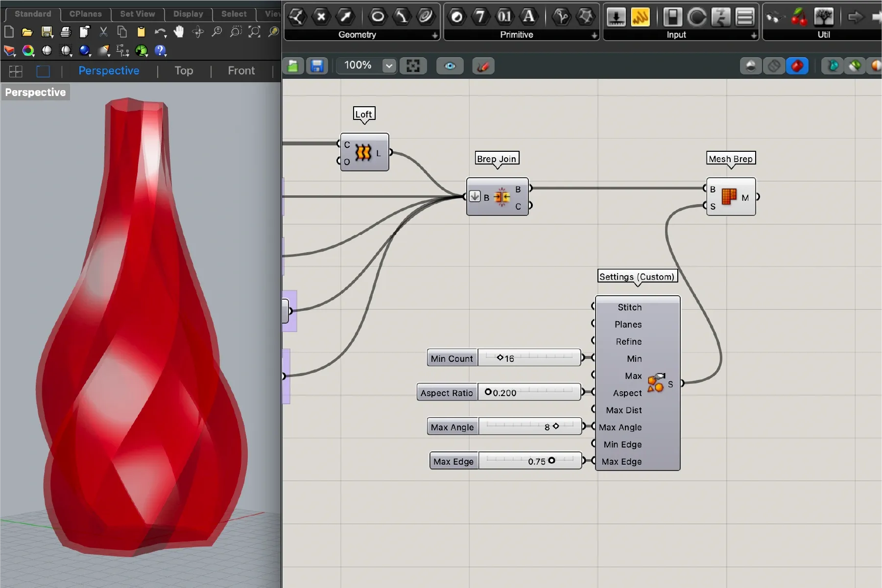
Converting to Mesh and Baking

One final step before export is model resolution tuning. We could bake directly from Brep Join (bake converts the parametric geometry into static Rhino geometry), but that can result in either too many polygons (heavy STL) or too few (low-definition print). Instead, we first send the solid to Mesh Brep and control polygon density with its parameters. After reaching a balance between detail and file size, we bake from this component and export as STL.

---

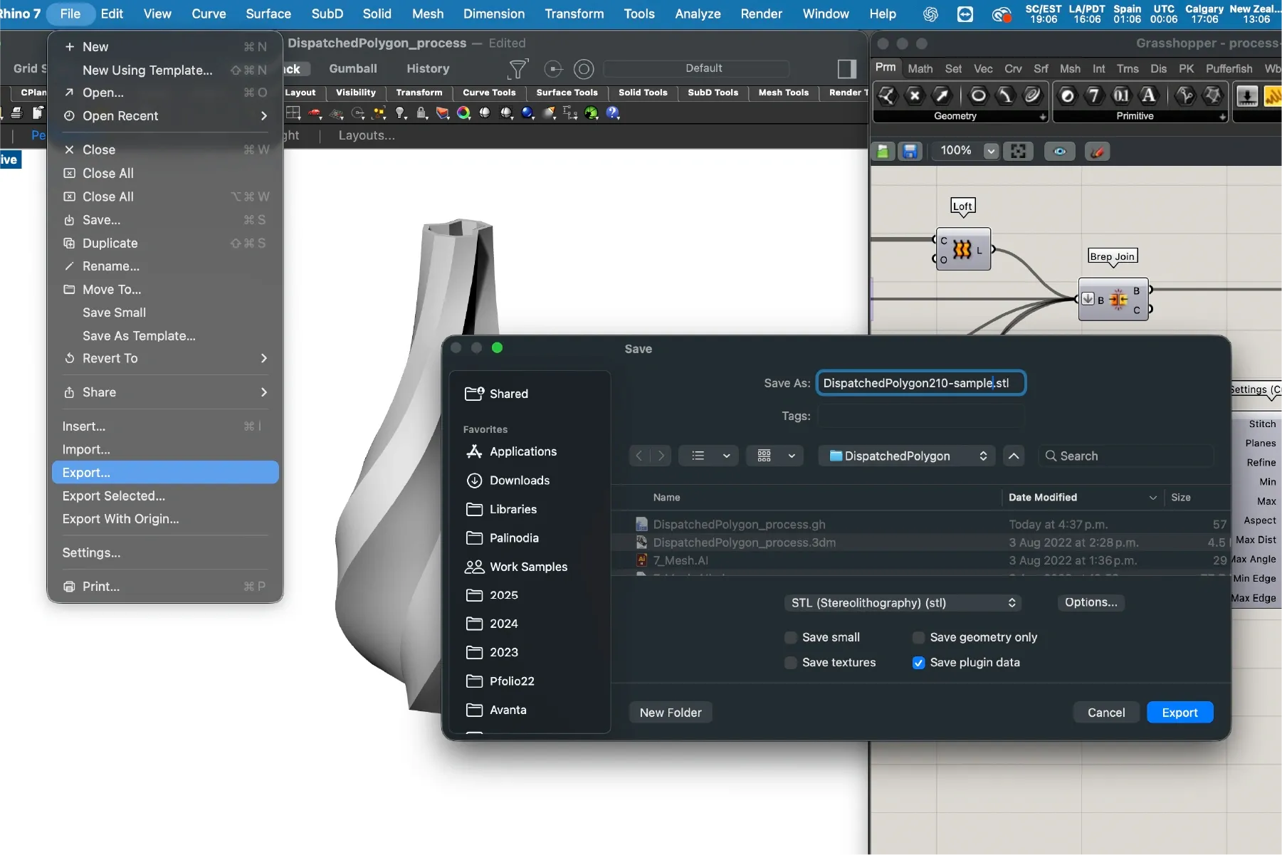
Exporting to STL

The object is now ready for export. In Rhino, we select the model, run Export Selected, and choose the STL format.

---

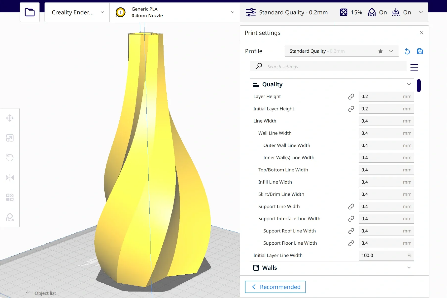
Slicing in Cura

3D printing is often more art than science. Every printer has quirks, and each model can require tuning. To print, we convert STL into gcode (the instruction format understood by printers). That conversion process is called slicing, and in this example we do it in Ultimaker Cura.

Cura lets us define layer height, print speed, infill, and more. For this model, we used 0.28 mm layer height, 15% infill⁴, 0.4 mm line width, and 52°C bed temperature. Through trial and error, these settings have worked well on our Ender 3 with our usual PLA filament⁵. The model is designed to avoid support structures⁶, simplifying print setup.

---

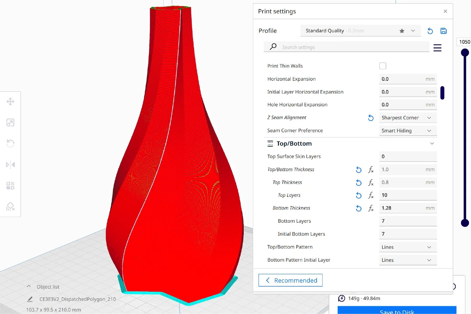
One additional detail that significantly affects print quality is Z Seam Alignment. Intentionally controlling where the seam (the point where the extruder moves up from one layer to the next) appears avoids random visual defects across the object. In the image below, the seam appears as a white line.

That completes slicing. We save generated gcode to a microSD card and load it into the printer.

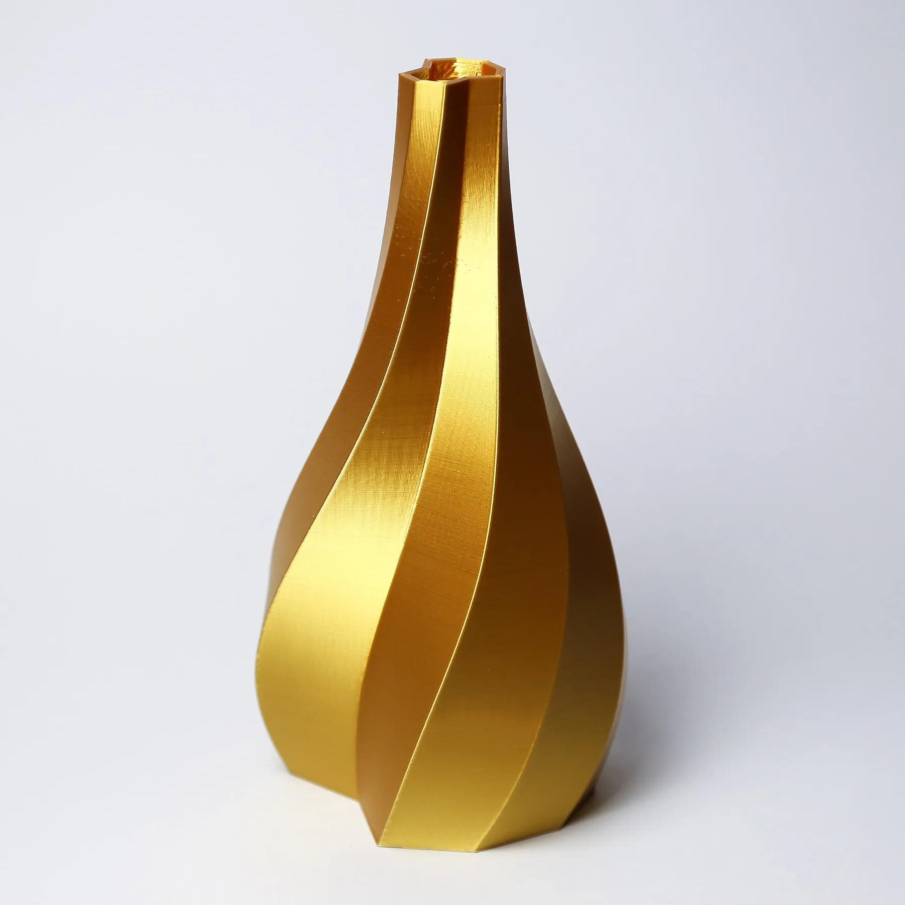
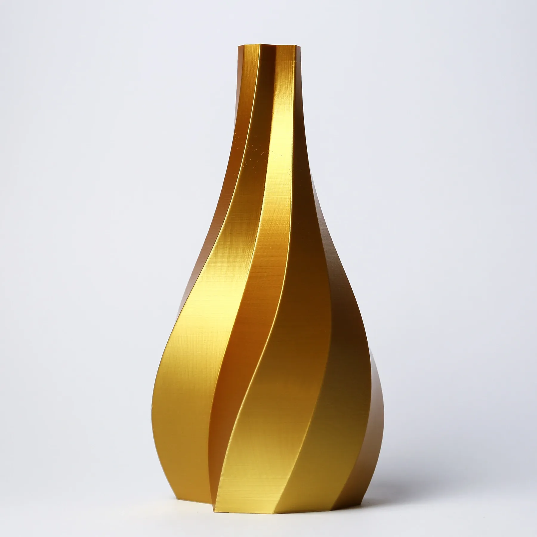
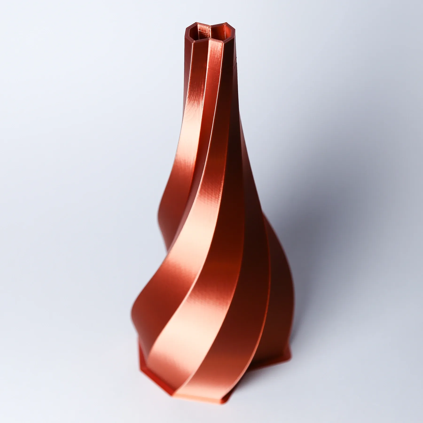
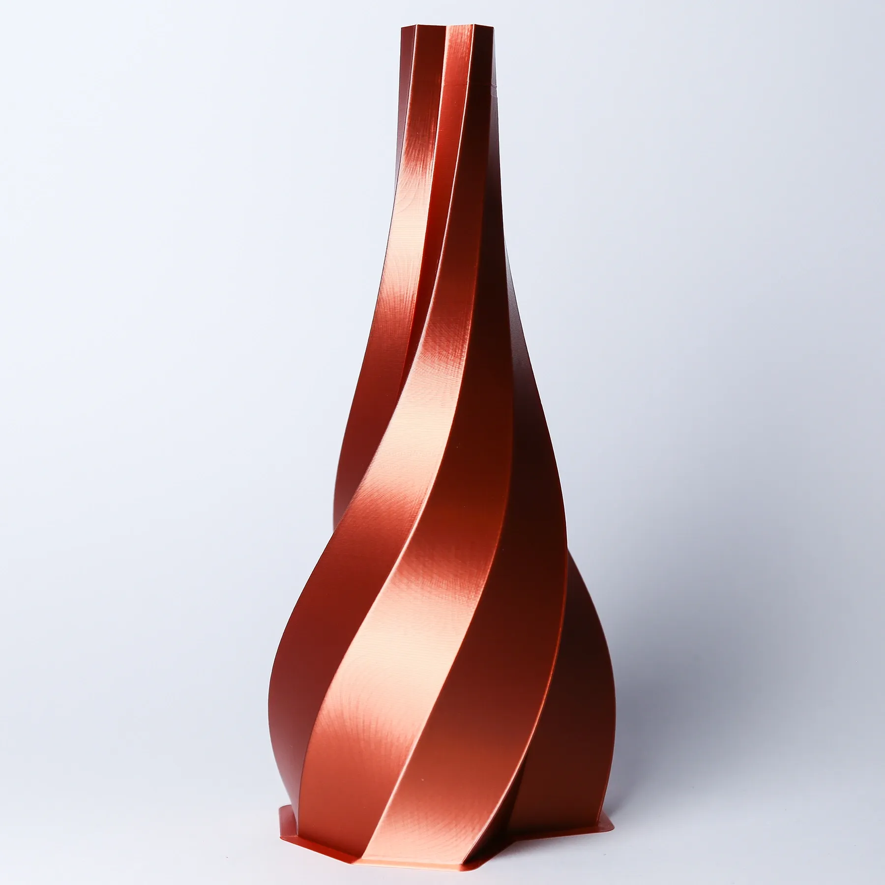
3D Printing

Starting a print is as simple as inserting the microSD card and selecting the gcode file. However, two practical factors make a big difference: carefully leveling the bed and monitoring the first layers (the shown prints can run 7 to 9 hours). In our experience, a glass bed and a extruder with a metal arm are worthwhile upgrades for adhesion and extrusion consistency.

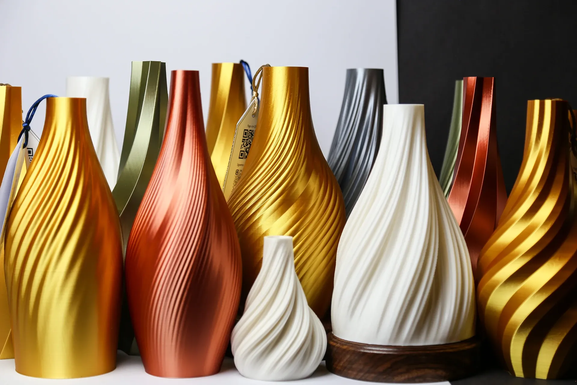
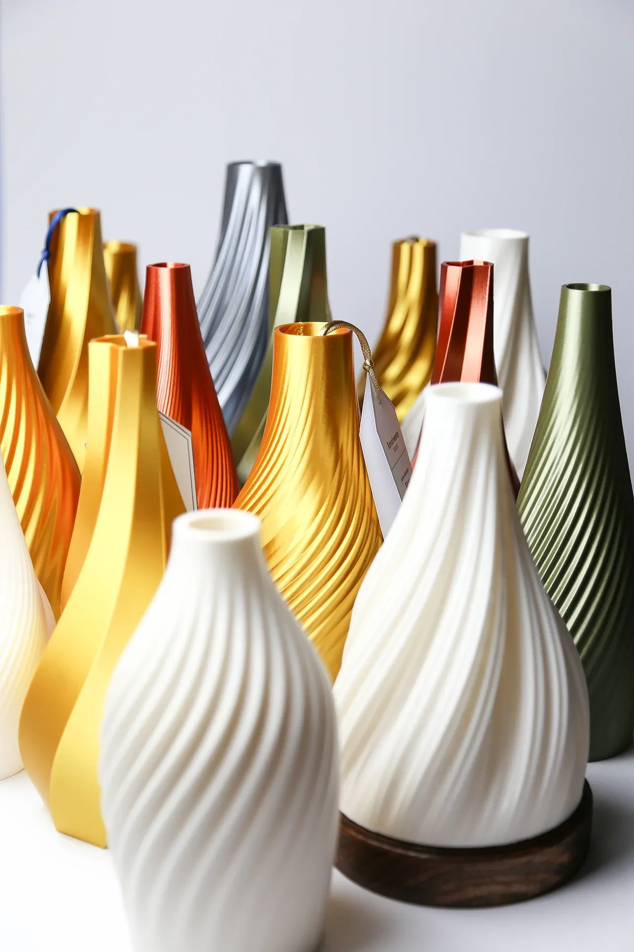
Final output:

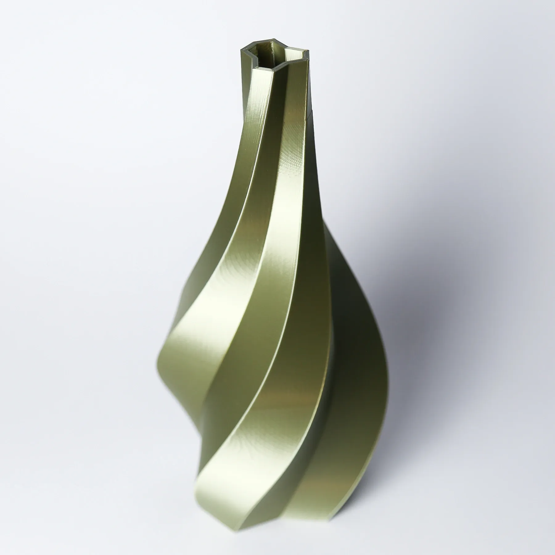
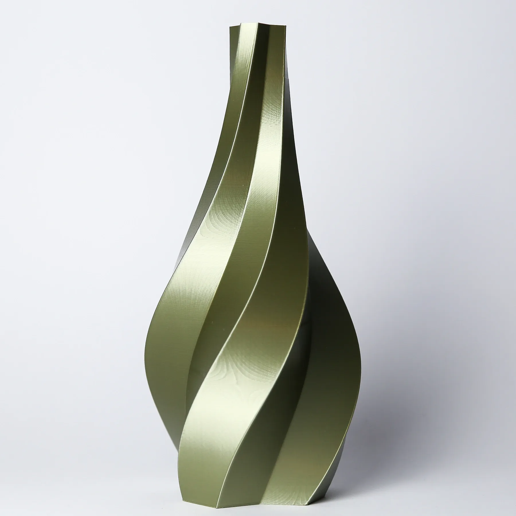
Other objects made with similar methods:

We hope this walkthrough of parametric design with Grasshopper and 3D printing was useful and inspiring. Parametric workflows open a wide creative space, letting us explore forms and structures that are hard to achieve with traditional methods. If you have questions or want to collaborate on a project, feel free to contact us.

Notes

Footnotes

1. Grasshopper is a plugin for Rhinoceros 3D, a widely used 3D modeling software in industrial design and architecture. Rhino is required to run Grasshopper, but this post focuses mainly on work inside Grasshopper. ↩

2. In this case, 0001 (no, no, no, yes): every vertex mapped to 0 goes to output B, and every vertex mapped to 1 goes to output A. Counting starts (counterclockwise) at the vertex shown on the X axis (red horizontal line). ↩

3. With Range, we define subdivisions inside a numeric interval. Here we split the 0 to 0.75 range into five divisions, producing six values (0, 0.15, 0.30, 0.45, 0.60, 0.75) used as rotation values for the stack levels. ↩

4. Infill is the internal structure of a printed object. 15% infill means the inside is not fully solid; a support lattice fills 15% of internal volume. Lower infill saves material and time, but can result in lower object strength. ↩

5. PLA (polylactic acid) is a common material for FDM printing (“Fused Deposition Modeling”, where filament is melted during extrusion). For decorative pieces like this one, we often use silk PLA. Non-sponsored recommendation: https://a.co/d/iPa77Ag ↩

6. Supports are temporary structures printed to hold overhangs. The second Graph Mapper (Gaussian curve) helps us control curvature intensity so supports are not needed in the print demonstrated in this post. ↩